How Much Prosody Can You Learn from Twenty Utterances?

Eric Keller / Brigitte Zellner Keller (Lausanne)

1 Introduction

Prosodic structures are marked by considerable complexity and are produced with substantial variability. At the same time, humans appear to recognize prosodic patterns quickly and surely. Seconds after tuning to a new radio station, we know whether we're listening to a sports report or a religious broadcast, even when the volume is too low to understand the words. In multilingual environments, just one or two utterances identify the language in use. If this observation on human prosodic perception is grounded in empirical fact, it should be possible to get a computer to identify, perhaps even learn, a given prosodic style in just a few utterances. Furthermore, we should be able to project this prosodic style upon new utterances. And by the examination of the internal workings of the prosodic model, we should be able to identify what distinguishes one prosodic style from another.

We found that it is possible to construct such a model with fairly simple statistical tools. By applying a set of multiple linear regressions to the relationship between linguistic and prosodic parameters, the essence of a prosodic style was captured in some twenty utterances. Specifically, the key prosodic parameters of duration [t, ms], fundamental frequency [F0, Hz] and intensity [I, dB] were reliably linked to automatically derived linguistic components of speech (segments, syllables, word groups and word group boundaries, etc.). This information was reversed and applied to new sentences by means of a speech synthesis device.

The methodology employed in this study, statistical models, is somewhat different from traditional linguistic methodology, since it pursues a different objective. In the linguistic tradition, the most desirable model is usually the one that is the most general. This principle extends the well-accepted scientific Principle of Parsimony (or "Occam's Razor"), which specifies that one should always choose the simplest and most general explanation of a phenomenon, i.e., the one that requires the fewest initial assumptions, leaps of logic, or further explanations. Specifying a given linguistic or prosodic rule (e.g., final syllable lengthening) for universal language use or for a certain set of languages is considered to be a much more desirable statement than specifying it just for one speaker, in a small set of utterances, or for one dialect of a given language. This serves to identify the "solid" components of language structures.

However, a problem arises with this approach when one wishes to specify the exact value of a rule, as when distinguishing its different uses in various languages, dialects, or speech styles, such as in a sociolinguistic or speech simulation study. In an emphatic use of Italian, for example, the precise degree of final syllable lengthening may well be notably different from that used in similar situations in English, French or German, although all four languages show the same basic phenomenon. This difference must be quantified somehow, not only by the presence/absence or frequency of use of a given rule, but also by its distinctive or gradient value, i.e., as long/short, or in milliseconds, or as a percent measure of some other duration. A process model or a prosodic model oriented towards a style- and speaker-specific characterisation of speech may thus have to be quite a bit more flexible and more detailed than a model for general language use. Such a model must not only specify which phonological rules should apply and with how much reliability, but also the gradient values that govern the rules' application.

Numeric models are thus essential for characterizing the fine details of language behaviour and for simulating speech behaviour over time ("process models"). In this class of models, the evolution of parameters over time is emphasized, a dimension which is not taken into account by traditional structural language descriptions (Zellner Keller 2002, 2003a, 2003b). While numerical approaches are particularly well-adapted to capturing significant details of the temporal evolution of quantitative parameters, qualitative aspects of prosody are of course not ignored. For example, just like descriptive models, numeric models must incorporate phonological and fast speech rules to be able to operate correctly.

Overspecification vs. Underspecification. Numeric prosodic modelling generally proceeds as follows: prosodic parameters (e.g., t, F0 and, I, henceforth the "dependent variables" or DVs) are derived from acoustic recordings, and relevant linguistic parameters (typically segmental and syllabic identity, position, number and context, henceforth the "independent variables" or IVs) are identified in the associated transcription. Numeric and/or logical relationships between linguistic and prosodic parameters (henceforth, "rules") are identified in various ways to create numeric and/or rule-governed models. Such models are then used to analyse and/or synthesize new stretches of speech and to fine-tune the model.

In this modelling process, two pitfalls should be avoided. A model based on very little data (e.g. one or two utterances) would be overspecified, that is, its rules would be too specifically oriented towards the input material at hand, and thus may not represent optimally prosodic relations in other, similar stretches of speech. To ensure a model's sufficient generality, a certain minimum number of observations of the IV-DV relation are needed. At the other extreme, a model can be too general for the purpose at hand. Since prosodic parameters differ from speaker to speaker, from speech style to speech style, and evolve even over the period of a given speech activity by a given speaker, it may not always be advisable to base a model on great amounts of speech material, since averages calculated on too much material may obscure the very distinctions of interest. The question thus arises as to the optimal amount of speech material required to satisfy the objectives of a given modelling effort. In our observations of the literature, this question has not yet received an extensive treatment. The present study furnishes some data relevant to this issue.

If only little material were needed for the key prosodic measures of duration, f0 and intensity, prosody modelling could be simplified. Instead of obtaining ever more data to feed an already sufficiently specified t-f0-I model, work could be directed at some of the more elusive prosodic indicators such as pauses, hesitations, turn-taking indicators, as well as semantic and pragmatic predictors of prosodic variation. These latter indicators may well take quite a bit more than twenty utterances to document, and will thus require considerable attention in the future.

This contribution has three main sections. In the first, our methodology is presented in some detail. This section is more extensive than usual to permit researchers less familiar with the numeric approach to undertake similar analyses themselves. Experienced researchers may wish to skip most of this discussion. In the second section, we discuss the results on two prominent MARSEC (Machine-Readable Spoken English Corpus, Knowles et al. 1996a, 1996b) speakers that were analysed with this system. Since numeric models can rapidly become complex, only a rudimentary statistical model without interaction terms is described here. Such a model is relatively easy to understand, all while providing initially satisfactory results. However, it is not an optimized model that could be used in a commercial synthesis. In the final part of the article, some suggestions will be made concerning how this class of models can be further improved by various techniques, and an outlook is given on further work that can be performed within this framework.

2 Method

2.1 Corpus, Speakers, Independent and Dependent Variables

Two British English speakers from the Machine-Readable Spoken English Corpus (MARSEC)[1] were chosen for this study. Both speakers are representatives of the received-pronunciation (i.e., the prestige/regionally neutral accent) form of British English (RP), and both are practiced adult speakers. The two corpus segments used here were (1) one and a half news bulletins spoken by Brian Perkins (BP) a BBC newscaster (the initial part of section B, 70 utterances, 7'522 segments), and (2) a portion of "Innocence and Design", the 1985 Reith Lecture presented by economist David Henderson (DH) (the initial part of section C, 70 utterances, 7'643 segments).[2]

The punctuation-free text transcriptions provided by MARSEC were marked up using common English punctuation rules. Signals from the corpus were subdivided at major tone group ("utterance") boundaries that are marked by double bars in the MARSEC prosodic transcription. With a few exceptions motivated by semantics and syntax, MARSEC tone markers were translated into periods, question marks, exclamation marks and colons. Commas were set according to English punctuation rules. The acoustic material from the two speakers was segmented using a computer-aided technique of placing automatic segmentation marks that are subsequently adjusted manually.[3] For this task, a phonetician was trained with a segmentation protocol defined in our laboratory (see Zellner 1998, Annex 4).

Independent variables. On the basis of the written versions of the text, punctuated and adjusted for hesitations and speech errors, a set of 19 linguistic descriptors was obtained automatically. Most of these descriptors have been shown to be of statistical relevance for the prediction of duration (Fant et al. 1991, Huber 1991, Keller 2002, Keller/Zellner 1995, Riedi 1998, Riley 1992) (number of descriptors is given in square brackets):

• Positional information [5] (segment position in syllable, syllable position in word, word position in minor phrase, minor phrase position in major phrase, major phrase position in utterance). "Major phrases" were text segments delimited by sentence markers and by commas. "Minor phrases" were delimited by punctuation marks as well as boundaries between lexical and grammatical words, as defined below. Such position indicators have been shown to be of relevance for the prediction of duration for French (Malfrère et al. 1998, Keller/Zellner 1995, Zellner 1996, 1998) and have also been successfully applied to German (Siebenhaar et al. 2001), as well as in various other languages (e.g., Campbell 1992 [English], Venditti/van Santen 1998 [Japanese], Febrer et al. 1998 [Catalan]).
• Quantitative information [5] (number of segments in syllable, syllables in word, words in minor phrase, minor phrases in major phrase, major phrases in utterance).
• Boundaries [1] (distinguished were: no boundary, syllable, lexical, minor phrase, major phrase, semicolon, period, question mark, exclamation mark and colon).
• Phonemic segment identity and lexical stress [6] (identity of preceding, current, and succeeding segments, lexical stress of preceding, current and succeeding segments).
• Part-of-speech [POS] membership [2] (the full POS classification according to the CUVOALD electronic dictionary,[4] and a simplified POS, where the CUVOALD classifications G Anomalous verb (e.g., auxiliary), Q Pronoun, R Definite article, S Indefinite article, T Preposition, U Prefix, and V Conjunction were set to "grammatical word" and the rest of the classifications (nouns, full verbs and adjectives) were considered "lexical words").

Dependent variables. Signals from MARSEC were denoised and enhanced using a generic technique furnished in the Pristine Sound software,[5] and they were converted to 16 kHz after appropriate low-pass filtering. The following DVs were obtained: (a) segmental duration as marked, (b) fundamental frequency extracted at 500 Hz by Praat's autocorrelation-based technique with default settings, except for a pitch ceiling of 250 Hz, and (c) intensity extracted at 500 Hz by Praat's intensity extraction, with the minimum pitch set to 75 Hz.[6] F0 and intensity curves were spot-checked for abnormalities and were found acceptable. For each segment, ten equally-spaced f0 and intensity values were derived from the extractions by interpolation, and mean values were stored for each segment. For ease of data manipulation, Praat's interpolated f0 values were used for unvoiced segments, although physically no voicing occurred, and logically no f0 value could apply. This manner of proceeding bore the risk of depressing f0 prediction values; however, this was considered acceptable, since (a) the interest of this study focuses on relative values and a depression in absolute predictions would have no bearing on the interpretation of the results, (b) prediction is unaffected for segments for which voicing is audible, and (c) the ultimate reduction in prediction proved to be minimal (see below). Pauses were not modelled in this study.

After generating IV and DV information, a computer-assisted technique was used to align the two sets of information. Specifically, the CUVOALD dictionary used for generating the IVs provides rhotic transcriptions (/kA:r/ for "car"), while the two speakers generally use non-rhotic pronunciations in the DV segmentations (e.g. /kA:/ for "car"). Since some r's were pronounced, adjustments were required to remove excess IV segment information. Similarly, some optional fast-speech rules, such as the suppression of schwa in "finally" or the deletion of the second /t/ in "contract talks" had to be accounted for. After each modification, IV positional and segment context information was automatically adjusted to reflect the segment's new status.

2.2 Multiple Regression as Applied to Prosodic Modelling

Modelling was performed with multiple least-squares linear regressions without interactions. In such a model, numeric relationships are calculated between a set of IVs and a given DV in such a way as to minimize the squared error along a straight prediction line (i.e., to minimize the squared distance from such a line). Multiple regressions are an extension of the simple linear regression of the form y = bx + a, where y is the dependent variable, b is a weight (or "coefficient") that multiplies the independent variable x, and a is a constant for the y intercept.

Figure 1. Normal probability plots for 4818 measures of segment durations, speaker DH. Left: original measures in seconds, middle: square-root transformed, right: log-transformed. Vertical axis: ordered response values, horizontal axis: normal order statistic medians. The data are plotted against a theoretical normal distribution in such a way that the points should form an approximate straight line. Departures from this straight line indicate departures from normality (NIST/SEMATECH 2002). In the present data, the square-root transformation provided the best approximation to a normal distribution.

In prosody, a simple linear regression could for example be applied to the problem of predicting duration from lexical stress in English. Since unstressed vowels tend on the average to be shorter than stressed vowels, a regression could be calculated in which x corresponds to lexical stress, with 0 for unstressed, 1 for secondary and 2 for main stress, and y corresponds to duration. The least-squares regression line in the x-y plane would run roughly from the bottom left to the top right. Multiple regressions extend this principle by calculating the x-y regression line from a group of predictors. Each IV-DV regression is calculated individually, and the weight of its contribution to the overall prediction line is optimized. In the application of multiple linear regressions, care must be taken to insure that the model's basic statistical assumptions are met. Primarily, data must be linearly distributed [7] (see Figure 1), distributions must be approximately normal, and extreme values not lying on the prediction line ("outliers") must be removed. Also, IVs showing multicollinearity (high intercorrelation) with other IVs must be selectively pruned, after considering their status from a theoretical point of view.[8]

In the present study, the data were subjected to the following procedures before applying regression analyses:

(1) Dependent variables were linearized. Various power transformations were applied separately for the three DVs and for the two speakers (log, square root, raw data, and power of 2), and the best transformation was chosen as judged with respect to the proximity to zero on a calculation of skewness. For both speakers, the best transformations in our data were the following: square root for segment duration, log for f0, and power of 2 for intensity.

(2) Independent variables were ranked with respect to their prediction for a given DV. This preprocessing step enables IVs for use as ordinal rather than nominal predictors, which considerably increases their power of prediction.[9] To illustrate with an example taken from our previous studies, the best predictor of segmental duration in French and German had been the phonemic identity of the segment (fricatives tended to be long, unaspirated stops tended to be short, etc.). Since there was no obvious articulatory or acoustic logic for ranking segments along the duration scale, our initial option was to treat segment identity on a nominal scale (as a set of discrete IVs). This was not very appealing, since one of the applicable regression mechanisms (regression for discrete or nominal values) was much less powerful than a regression for ordinal or scale values, and another procedure, the frequently employed binary regression tree (e.g., Riedi 1998, Klabbers 2000) required quite a bit more data, due to the "sparse-data problem".[10] A multiple regression for the modelling of duration based on simple nominal values would explain only about 10-20% of variance, while ranked regressions for the same data set generally explain more than 50%, and sometimes as much as 79% of variance (Zellner 1998).

In our previous work, segments were thus recoded as members of "duration groups" (Keller/Zellner 1995). To counter the arbitrariness inherent in the constitution of such groups, Zellner (1998) proposed a grouping on the basis of purely quantitative criteria, a solution which was subsequently applied to German as well (Siebenhaar et al. 2001). This categorisation process was quite successful, yet it also led to a certain loss of predictive power because of the grouping of values. Also, while a specific grouping may be satisfactory for one IV-DV relationship (e.g., the current segment identity - duration relation), it may not be optimal for another (e.g., the relation between the identity of previous segment and the duration of the current segment).

Table 1. Illustration of recoding of IV values

Comment: IVs (for illustration here: segments) are initially assigned arbitrary codes for computational manipulation and for compatibility with SPSS. They are then ranked according to their average prediction on the IV-DV relationship in question. Since the DVs are themselves linearized by a given transformation, the transformed value is used as the rank number (IV1-3_trans). This recoding procedure has the effect of transforming nominal IVs into rank-order IVs, which substantially increases their predictive power. The sample utterance "how are you" is recoded here.

In the present study, optimal ranking of IVs was achieved by placing corresponding linearized average DV values into IV prediction cells. For example, the short vowel /I/ has an average duration of 58 ms in the data for speaker DH. Since this is a duration, its linearized value, i.e., the square root of 0.058 s, or 0.2409 was placed in the duration-predicting IV cell for this segment. If a numeric value was absent from the corpus (e.g., if stress 0 and stress 2 were attested, but stress 1 was not), the interpolated value was taken (i.e. (mean_stress0 + mean _stress2)/2). If a nominal value was unattested, but exists in the language (such as /Z/), the DV's mean value was used as a predictor value in the simple version of the algorithm used for this study.[11] All IVs were re-coded in this manner, separately for each IV-DV relationship (for an illustration, see Table 1). This means, for example, that there is one ranking for the current segment - current duration relationship, but a potentially different ranking for the relationship between the identity of the preceding segment and the duration of the current segment.

To sum up, the present study takes the ranking logic to its limit and preserves the greatest possible amount of predictive power by abandoning categorisation of IVs, by treating each IV-DV relationship separately, and by letting the data itself determine the ranking, instead of imposing groups preconceived on theoretical grounds. Furthermore, the approach is generalized here to f0 and intensity.

(3) Outliers were examined individually, and modifications to the source data were applied as judged appropriate. Outliers were defined as data points lying two RMSEs or more above or below the predicted value for the given data point. (See below for a definition of the RMSE). The prediction model was recalculated after an inspection and the potential removal/modification of outlier values.

(4) Variable pruning. After the calculation of an initial set of regressions for the two speakers, IVs showing multicollinearity were removed with the aid of the stepwise procedure provided in SPSS. This assured the required degree of orthogonality in the predictor variables (all of which are related to DVs to a statistically significant degree, p<0.05), and it served to stabilize the regression coefficients. After this pruning step, IVs shown in Appendix I were retained. It is noted that the list is somewhat different for the two speakers.

2.3 Evaluation and Precision

The evaluation of prosodic models. The performance of prosodic models can be assessed by several objective and subjective indicators. Typical objective measures are the correlation between predicted and measured values on pre-existing (model-feeding) as well as novel data, the percent of variance explained, derived by squaring the correlation coefficient, RMSE, the root mean-squared error on the prediction (akin to the standard deviation from the mean), and the bias of the prediction, i.e., the degree to which the model systematically under- or overpredicts target values.[12] [13] Arguably the most powerful objective indicators are RMSE and bias. RMSE compensates for differences in corpus size, and it is affected by bias, which is left aside by correlation-based statistics. A separate examination of bias may point up structural limits or basic deficiencies in the model.

While these indicators are useful to the model builder, it is hazardous to use them to compare models from different speakers, different speech tasks and different languages, since they vary considerably as a function of speech task and regularity of the subject's speech behaviour, and since they do not necessarily reflect perceptual impressions. In fact, it is quite difficult to accurately assess the "quality" of any prosodic model (see Sonntag 1999, for an extensive treatment of this issue). In our work on exceptionally careful speakers of French and German, for example, Pearson r's of 0.8-0.9 were attained for segmental durations (r = .870, RMSE = 18 ms, reported for French by Zellner 1998 and Zellner Keller 2002; and r = .84 reported for Swiss High German, [14] Siebenhaar et al. 2002). When such timing models are combined with measured F0s and implemented in a speech synthesis system such as Mbrola, [15] the rhythmic component sounds quite convincing. With some other speakers, other languages and in less formal speech, however, much lower coefficients (e.g., r's of 0.6-0.8) have also been encountered using the exact same methodology. Yet such objectively "weaker" models may perform also reasonably well when driving a speech synthesis system.

This has led to the notion that prosodic models should be evaluated via speech synthesis. It is argued that more natural, holistic percepts can be created from several prosodic sub-models, minimally one for timing and one for melody, and that such percepts can be compared to that obtained from human speech. This introduces several new problems, however. Most importantly, the output combines effects and degradations introduced by the prosodic module with those produced by the downstream signal generation module. Since signal components are often quite deficient, this leads to dubious perceptual comparisons between two very different entities, artificial and human speech. Furthermore, the long-term value derived from fairly costly perceptual tests is questionable, since speech synthesis systems are in constant evolution, and judgements obtained one year may be outdated the next. Consequently, only prosodic output via a specific signal generation module is compared here, and we are circumspect about percepts derived from speech synthesis, even though we favour such implementations for the interactive development and testing of speech models (Keller 1997, 2002, forthcoming).

Precision. A final concern in prosodic modelling is measurement precision. Although computer programmes will perform their analyses according to an exact set of criteria, the criteria themselves may not be defined (or easily definable) with sufficient completeness or complexity. For this study, human intervention was applied at five points: (1) the initial identification of predictor variables, (2) the phonetic segmentation of the acoustic signal, (3) the alignment between the "default" (dictionary-and-rule-based) phonetic segment sequence and the actually produced phonetic segment sequence, and (5) the selection of input parameters for final statistical analyses.

3 Results

Two research questions were examined here:

1. How much data is required to build a reliable t-f0-I prosodic model?
2. How well do minimal t-f0-I prosodic models project to novel data?

In the following section, results for speaker BP are given first, and for speaker DH second.

3.1 Modelling the Original Data

To examine the first issue, 50 models per DV were calculated over domains of various sizes. The first model was calculated on the basis of just two contiguous utterances (1 and 2), the second on the basis of three (utterances 1, 2 and 3), through to the last model which was calculated on the basis of the 51 initial utterances (1...51) of continuous speech by the two speakers. Models were calculated separately for the three dependent variables t, f0 and I.

The results for the Pearson correlation coefficient r and RMSE show that the models stabilize rapidly beyond the fifth utterance (Figure 2). Approximate stability is attained by models that are based on twenty utterances or more. The stability estimates are similar for the two speakers, even though the model fits for BP are better than those for DH. The exact measures were as follows for model 20, based on 21 utterances: (Speaker BP) t, r = .735, p<.001, RMSE = 24 ms, bias = 2.3 ms; f0, r = .502, p<.001, RMSE = 2.55 semitones (16.7 Hz), bias = 1.24 Hz; I, r = .790, p<0.001, RMSE = 4.82 dB, bias = -0.17 dB. (Speaker DH) t, r = .686, p<.001, RMSE = 28 ms, bias = 2.7 ms; f0, r = .294, p<.001, RMSE = 3.76 semitones (25.4 Hz), bias = 2.65 Hz; I, r = .721, p<0.001, RMSE = 5.56 dB, bias = -0.23 dB.

Since the model for fundamental frequency predicts values for both voiced and unvoiced segments, even though only voiced segments provided reliable input data and unvoiced data were interpolated, f0 predictions were potentially depressed in comparison with predictions for segmental durations and intensities. However, a separate run for the voiced segments of model 20 showed few if any improvements. Correlations r's for voiced segments (N=602) were .549 for BP (marginally better) and .294 for DH (N=742, unchanged), and RMSEs were 2.47 semitones (15.7 Hz) and 3.6 semitones (24.2 Hz) respectively, both marginally better.

Since bias captures the degree to which a model over- or underestimates target values, it was interesting to examine the relationship between bias and RMSE (Figure 3). There were strong correlations between RMSE and bias for all parameters (t: r=.906, f0: r=.988, I: r=-.904), indicating that in this data set, bias accounts for nearly all of RMSE variation.[16] However, the percentages of the RMSE accounted for by bias were not excessive (means of bias as a percent of RMSE for 50 models and the two speakers: t: 9.8% and 10.0%, f0: 7.3% and 10.2%, I: 3.5% and 4.0%). This analysis shows that the models for the two speakers tended on the average to underestimate duration and fundamental frequency, and to overestimate intensity. This can probably be related to the physical and physiological nature of the scales involved. In normal speech, segmental duration is open-ended at the top but close-ended at the bottom, fundamental frequency shows more range above median activity than below, and intensity shows the inverse tendency.[17] This is reflected in the relationship between the mean and the median, where BP, for example, shows a median lying below the mean for duration (median: 48.6 ms, mean: 50.0 ms) and fundamental frequency (median: 100.7 Hz, mean: 102.2 Hz), but a median situated above the mean for intensity (median: 72.7 dB, mean: 71.8 dB).

A further observation is of interest. The closeness of fit for some of the small-footprint models (e.g., model 7 for BP, based on eight utterances and 779 (BP) / 978 (DH) segments, or model 6 for DH, based on seven utterances) is especially strong for duration and fundamental frequency (see Figure 2). Also a hint of a "counter-effect" is visible for f0 around models 16 and 13, respectively. It is possible that a rather good short-term fit could be based on just seven to eight contiguous utterances. In contrast to the stable long-term model visible for pools of 20+ utterances, this short-term model could possibly represent an optimum for capturing changing prosodic trends within ongoing speech activity.

Sliding-window model fits for 70 sentences appear to bear out the similarity of results for short- and longer-term analyses. In this analysis, a first set of short-term models based on a sliding 8-utterance window, and a second set of longer-term models based on a sliding 20-utterance window were calculated. For each speaker, all possible models were constructed for a total of 70 continuous utterances (Figure 4). In several tasks, the 8-utterance models fit the data better than the longer-term 20-utterance models, particularly for BP, both in the sense of reflecting more local variation and by reducing the RMSE somewhat. In other tasks and particularly for DH, the results were mixed, but the longer-term models never showed any clear superiority over the short-term models.

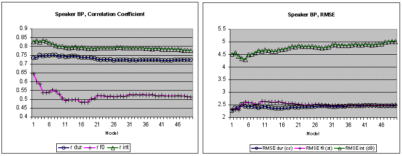
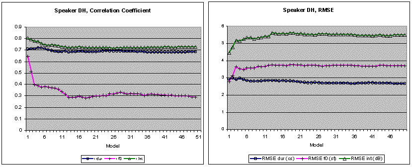
Figure 2. Correlation coefficients and RMSEs for 50 models of increasing domain, where model 1 is based on utterances 1...2, model 2 on utterances 1...3, and model 50 is based on utterances 1...51. Left: Closeness of fit as measured by the correlation coefficient r between predicted and measured mean segment values for segmental duration, fundamental frequency and intensity (with r, higher is better). Beyond the 20^th utterance, the model fit is approximately stabilized for all three measures and for both speakers. Right: In terms of the RMSE (where lower is better), the fit appears to stabilize even earlier, on the basis of fewer utterances. The stability estimates are similar for the two speakers, even though the model fits for BP are better than those for DH. The N for the first 20 utterances was 1'962 and 2'331 phonetic segments for BP and DH respectively.

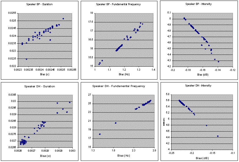
Figure 3. The relationship between RMSE and bias for the two speakers. Strong correlations are visible for all parameters (t: r=.874 and .979, f0: r=.989 and .997, I: r=-.979 and -.999, all p<0.001), suggesting that bias accounts for nearly all of RMSE variation. Since bias = mean(predicted_i -observed_i ), positive-going values correspond to underestimations and negative-going values to overestimations. In both cases, greater divergence from zero corresponds to greater degrees of under- or overestimation. In all conditions shown here, bias accounts only for a small proportion of total error, typically less than 10%. Also, bias does not account for residual (unsystematic or otherwise unaccounted for) error.

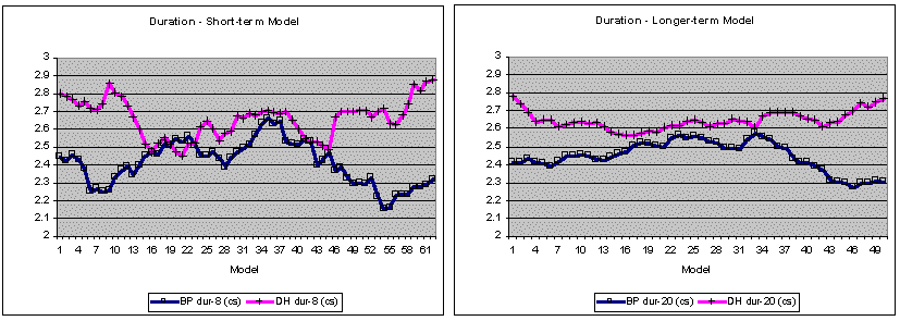
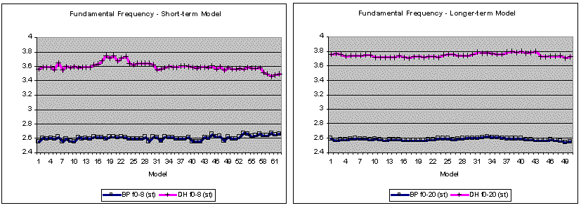
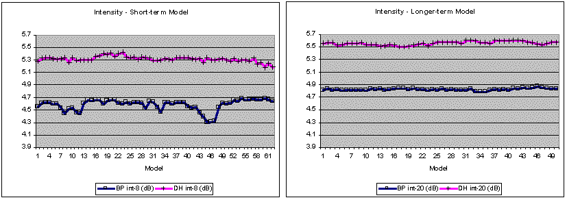
Figure 4. Model fits of 70 utterances of continuous speech, as estimated by the RMSEs on 8- and 20-utterance sliding window analyses. In some tasks, short-term models fit the data better than longer-term models (with RMSE, lower is better). Since RMSE variation reflects primarily bias (as confirmed for the sliding-window models) and thus represents over- and underestimations, the variations shown here correspond primarily to the presence of excessive values in the data. E.g., the increase of duration RMSEs in the first part of BP's first news bulletin (models 8-35) reflects the presence of a substantial number of particularly long phonetic segments, as verified manually.

Since RMSE variation was again found to reflect primarily bias and thus captures small over- and underestimations, the variations shown here probably correspond to the presence of excessive values in the data. For example the stretch of high-duration RMSEs in the middle of BP's speech material (roughly, the middle of the first news bulletin) suggests that in those places, the model underestimates duration in the observed data, which in turn suggests the presence of an exceptionally high number of particularly long phonetic segments. This was confirmed by a visual inspection of the raw and bias values (not shown here). At the beginning of the news bulletin (models 0-7), average bias decreases briefly, to be followed by a long rise (models 8-35), and during its last part (models 36-42), bias was seen to decrease. (The first news bulletin ends on utterance 49.).

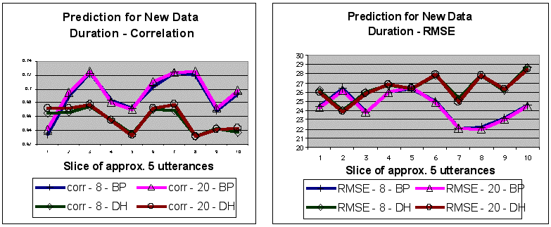
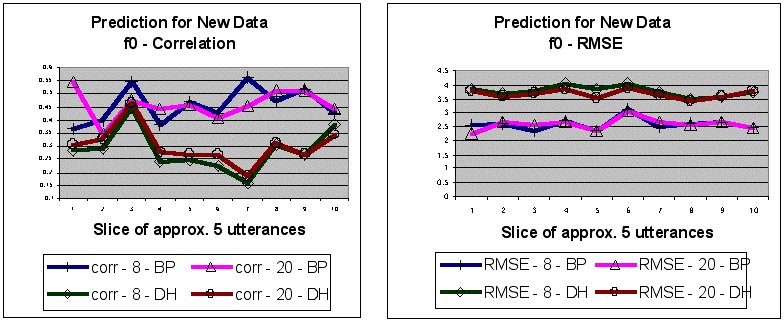
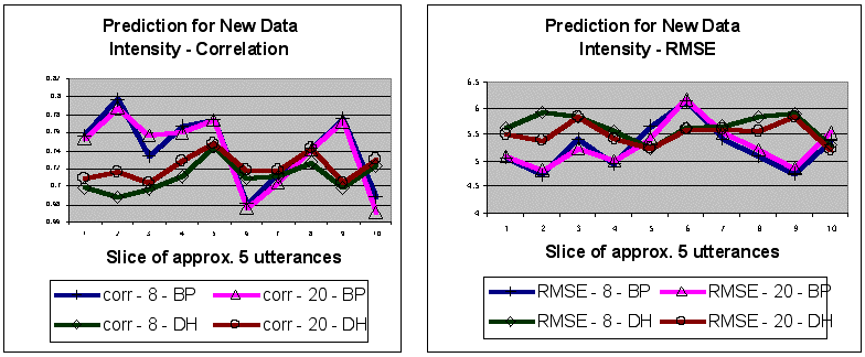
Figure 5. Model fits for new data as measured by the correlation r and RMSE between produced and predicted prosodic values. Model fits are weaker than for the original data, and BP's model has greater predictive strength than DH's models. Models based on 20 utterances furnish only marginally better predictions than those based on eight utterances (average of 1.3% for correlations, 0.9% for RMSEs).

In conclusion, it seems reasonable to suggest that a t-f0-I prosodic model for news and lecture material can furnish useful short-term information based on just eight utterances, or less than 1000 segments, while a still very compact 20-utterance model can provide a stable estimate of longer-term behaviour of these three prosodic parameters.

3.2 Modelling Novel Data

Correlations and RMSEs. To examine the models' ability to generalize to novel speech material, 8- and 20-utterance models were trained on the two speakers' initial utterances in the corpus and were applied to the speakers' respective utterances numbered 21-70. Only data from the training set was used in the ranking procedure for the IV-DV relationships used in the training models.

The new speech material of 50 utterances was subdivided into equal slices of about five utterances each. Each slice was 556 segments long for BP and 591 segments long for DH. Correlations and RMSEs were calculated between predicted values and prosodic data extracted from the original files (Figure 5). Results showed that model fits were weaker than for the original data, but for the most part were still in the useful range. RMSEs were less strongly correlated with bias (r_t = .460, r_f0 = .415, r_I = .049, average of two model types, both subjects), suggesting that some of the divergence between produced and predicted values was probably due to differences between the model's source data and the novel data, not to systematic model bias. In line with BP's better-fitting models for the original data, this speaker's model had stronger predictive power for new data than did the models based on DH's material. Models based on twenty utterances furnished only marginally better predictions than those based on eight utterances (an average of 1.3% improvement for correlations and an average of 0.9% improvement for RMSEs).

Missing data were calculated for eight new utterances on the basis of eight and twenty utterances (Table 3). It is recalled that the missing data for numeric IVs (e.g., stress levels) are interpolated and that average values are substituted for nominal IVs (e.g., segments). Since interpolation was necessary for 5% or less of predicted values, and since no substitution of averaged values was necessary, it can be concluded that missing data did not play a major role in this data set.

Table 3. Missing Data

In general it can be concluded from this set of experiments that t-f0-I models based on as few eight contiguous utterances generalize satisfactorily to new speech material from the same speaker and in the same speech style, as long as the original fits are satisfactory. For example, BP's original models for fundamental frequency showed a relatively low correlation r of around 0.5 with an RMSE of around 2.5 semitones (Figure 2). In their application to new material, the correlations dropped to around 0.45, but the RMSEs stayed at about 2.5 semitones. By contrast, DH's models for fundamental frequency showed very low correlations r's of about 0.3 and considerably higher RMSEs of about 3.8 semitones on both old and new material. At these levels, the models' predictive capacity is so diminished that their usefulness can be questioned. This suggests that initial speaker selection plays a more crucial role in assuring high levels of model fit than increased amounts of data.

Speech Synthesis. In a second test of the models' ability to generalize to new data, two passages were synthesized on the basis of the 8- and 20-utterance models for the two speakers. The first was a Hello World message, the second was the British version of the Northwind Passage.[18] Only predictions for segmental duration and fundamental frequency were used. Four fundamental frequency values were generated by interpolation from the single predicted value per segment, and a cubic spline function was applied to smooth the f0 curve. Pauses were simulated by static rules (end of major breaks: 100 ms, utterance final: 600 ms). Durations were linearly lengthened somewhat (maximum: 5%) to facilitate perception and judgement.[19] Outputting was effected through Mbrola with the "en1" diphone database,[20] and was subsequently denoised and filterband enhanced with the Pristine Sound software, before being converted to MP3. The sounds are available at our website.[21]

Without systematic perceptual testing, it is hazardous to form judgements concerning these sample files. At the same time, the main conclusions of the objective evaluation do appear to be borne out. They are:

• An interesting default t-f0-I prosodic model can be based on very little speech material using the methodology described here.
• There are few differences between models based on eight and twenty utterances, with the possible exception of f0 prediction.
• The better-fitting models based on BP's speech do appear to sound a bit better than those based on DH's speech material, particularly with respect to fundamental frequency.
• Some of the stylistic differences between BP's and DH's prosody can be identified in the synthesis by listeners familiar with the speech patterns of the two speakers, notably DH's considerable f0 modulations.

4 Outlook for Further Research

It was found that simple linear regression models for t, f0 and I, based on eight and twenty consecutive utterances of news bulletins and prepared lecture presentations showed good stability, satisfactory prediction for novel material, as well as closeness of fits comparable to those reported by other researchers for much larger corpora. For example, the RMSEs for duration data in our two speakers ranged from about 21-29 ms for about 2000 segments. Klabbers (2000: 70), using classification trees established on the basis of phonetic principles, reported RMSEs ranging from 19 to 27 for duration data on Dutch (RMSE 27 ms, 12'948 segments), German (RMSE 19 ms, 24'240 segments) and French (RMSE 25 ms, 7'143 segments). We saw that beyond the 20^th utterance, the variable of greatest impact was not the size of the data set, but the selection of the speaker (e.g., mean duration RMSE_n=8 for BP: 24.0 ms, DH: 26.5 ms). Also, closeness of fit varied over short stretches of speech, suggesting that a locally-adapted model may sometimes be preferable to a models based on long-term behaviour.

It may be possible to further optimise this type of model:

1. Predictors. While the current, easily obtainable set of independent variables shows fairly good predictive power, it does not exhaust the list of useful prosodic predictors. Some obvious variables left aside in this study relate to semantic prominence and stress. Manually-marked or upstream-generated semantic prominence inputs would quite likely improve the power of the model. Similarly, stress was treated as a lexical phenomenon here, while phrase-domain stress rules would probably be better predictors for running English speech.
2. Interactions. The modelling of interactions was left aside here. Yet many independent variables clearly show interaction effects. For example, in vocalic portions of a syllable, stress has different effects on segmental duration than during consonantal portions. There thus exists an "interaction" between stress and segmental type, as the two exert their combined effect on duration. In our French synthesis, some of these deficiencies were "patched up" by supplementary rules. It would be preferable to incorporate interactions right into the overall model, for example by including a set of contextually inspired predictor variables, or by having the multiple regression algorithm model interactions directly.
3. Increased exposure to absent predictors and to missing data. As mentioned in footnote 11, it would be short-sighted to believe that the occasional erroneous calculation based on a missing data point or the absence a rarely-occurring predictor does not matter to a careful listener. At the same time, simple calculations of probabilities of occurrence for rare phonetic and prosodic data indicate that even sizeable data bases (e.g., in excess of 100'000 segments) cannot provide actual data points for every phonetic and prosodic contingency (for further discussion of this point, see Portele 1998, Möbius 2001 and Keller 2002). Consequently, more advanced models would have to include a sophisticated logic to deal with missing data, based on a theoretically and empirically informed analysis of observed IV-DV relationships.
4. Nonlinearities. Multiple linear regressions are efficient and relatively unambiguous in their application, but they require linearity and approximate normality of distribution in the dependent variable. In our work on t, f0 and I, this has not posed any insurmountable problems, but the case may be different for the prediction of other prosodic parameters (pauses, turn-taking signals, etc.). If considerable nonlinearities are observed, numeric modelling techniques more adapted to non-linear data (such as neural nets) may be called for (for the application of neural nets to prosodic parameters, see Campbell 1992, Pfister/Traber 1994, Traber 1992, and many subsequent authors). The neural net approach becomes of particular interest if there is evidence of non-gradience in the prosodic parameter of interest, e.g., when prosodic parameters act as "edge markers" in speech, rather than as continuously present parameters in need of quantity specification (as with t, f0 and I).

It thus appears that the relationship between size of data base and prosodic model is largely a function of the parameters involved. From the present results it can be concluded that the fundamental behaviour of frequently-observed continuous parameters such as t, f0 and I can profitably be modelled on the basis of relatively small amounts of data, at least in read material such as news bulletins and professionally delivered lectures. More data per se did not improve the model fit or render it more stable. On the contrary, models based on more than an optimal amount of data may well be incapable of capturing the very detail of interest in specific speech and speaker styles.

This suggests that small-data models could well serve as default models for the simulation of individualized prosody, and that sophisticated ways (typically extra parameters and specific rule sets) should be devised to deal with the deficiencies induced by missing data. Particularly, infrequent and inconsistently used "marker" parameters would probably require specific well-targeted investigations of wider data sets before they could be modelled adequately. Building a series of well-adapted small-footprint models may well say more about the individual use of prosody in specific speech situations than building a single model on the basis of a great deal of data.

Acknowledgements

Mr. L. Wiget is thanked for his diligent work with manual segmentation and for his assistance in the development of text analysis routines for English. Cordial thanks are also extended to Antje Schweitzer (IMS Stuttgart) for detailed and insightful comments on an earlier draft of this paper. This research is supported by a Swiss OFES grant under COST 277.

Notes

1 MARSEC is available from www.rdg.ac.uk/AcaDepts/ll/speechlab/marsec . [back]

2 According to the BBC, Brian Perkins is originally from New Zealand and came to the U.K. in his early twenties. His news-reading style is widely acclaimed. The U.K. economist David Henderson has held various academic posts and appointments in U.K. and international organisations. This is not the same person as the U.S. economist David R. Henderson.[back]

3 Thanks are given to Dr. Karlheinz Stöber, now at BKA, Wiesbaden, Germany, for the use of his dsp_dtwalign algorithm in this context.[back]

4 CUVOALD: Computer Usable Version of the Oxford Advanced Learner's Dictionary (1992). Available from ftp://svr-ftp.eng.cam.ac.uk/pub/comp.speech/dictionaries/.[back]

5 Available at http://www.accuratesound.net.[back]

6 Praat is available for free at http://www.praat.org.[back]

7 This is a particularly stringent requirement for speech simulation experiments. If a linear prediction is made for prosodic values with a non-linear distribution, the strongest and most audible predictions will typically be among the most erroneous. [back]

8 In its stepwise procedure, SPSS removes variables based on multicollinearity and contribution to the explanation of variance. However, Howell (1999) emphasizes the importance of basing the removal of variables not only on statistical, but also on theoretical considerations. For example, the simplified lexical/grammatical POS (obviously) showed multicollinearity with the full POS information, as distinguished by the CUVOALD dictionary. After considering the behaviour of the two IV's throughout the data set, simplified POS IVs were removed when they co-occurred with full POS IVs, even though according to SPSS, both could have remained in the equations.[back]

9 Ordinal predictors behave just like scale predictors in normal multiple regression analyses.[back]

10 The "sparse data" or "LNRE (Large Number of Rare Events)" problem refers to the pervasive and difficult issue that certain linguistic features or elements are far less frequent than others and that any combinatorial information is difficult to obtain for the less frequent elements (Van Santen 1997, Van Santen/Shih 2000, Keller 2002, Möbius 2001). For example, /t/ is a very frequent sound in English, while /Z/ (as in "measure") is very rare (Roberts 1965). Consequently, it is difficult to collect enough data to illustrate how /Z/ behaves in all possible segmental combinations.[back]

11 Missing nominal values can be a system's Achilles heel: the smaller the data set and the more exclusive the set of prediction features that are employed, the more occurrences of missing nominal values and essentially meaningless predictions there will be. Contrary to what might be expected, a careful human listener does not simply pass over the occasional erroneous predictions induced by an expedient use of mean values. Sophisticated rules are required to deal with the missing data problem in more advanced models (see "Outlook for further research", below). In the current study dealing with the prediction of the common parameters t-f0-I from a set of fairly pervasive linguistic features, missing nominal values did not pose a particular problem (see below). [back]

12 RMSE is defined as sqrt(sum_i...n (observed DV_i - predicted DV_i)²)/n) and bias is defined as sum_i...n (observed DV_i - predicted DV_i)/n. [back]

13 Several other measures are possible (e.g., a relative RMSE), but no convincing case has been made for their use (see discussion in Klabbers 2000).[back]

14 Combined modelling of segmental and pause durations.[back]

15 For Mbrola see: http://tcts.fpms.ac.be/synthesis/mbrola.html.[back]

16 It is not necessary for bias to correlate with RMSE. As the deviation from a prediction changes, both RMSE and bias change, but not necessarily in the same direction, since RMSE is based on a squared error estimate and bias is based on a direct error estimate.[back]

17 Assuming skew-optimized scales for the three variables, as discussed above.[back]

18 The Hello World message is: "Hello world, how are you, I'm a simple {eight, twenty}-utterance prosodic model, trained on {speaker's name}, speaking through Mbrola." The Northwind Passage exists in a North American and a British version (available at http://www.alt-usage-english.org/north_txt.html). The North American version of the Northwind Passage was used in the early 1980s for an evaluation of the MITalk system (http://www.mindspring.com/~ssshp/ssshp_cd/ss_mit.htm).[back]

19 Native English listeners unfailingly considered the unlengthened versions to be too rapid, a phenomenon that may be attributed to the limited quality of the resynthesis system.[back]

20 The en1 database was provided by the Edinburgh team distributing the Festival project: Alan Black, Paul Taylor, Roger Burroughes, Alistair Conkie, and Sue Fitt. http://www.cstr.ed.ac.uk/projects/ festival.html.[back]

21 http://www.unil.ch/imm/docs/LAIP/LAIPTTS_pros_footprint.htm . [back]

References

Campbell, William N. (1992): "Syllable-based segmental duration". In: Bailly, G./Benoit, C. (eds.): Talking Machines. Theories, Models, and Designs. Amsterdam: 211-224.

Fant, Gunnar/Kruckenberg, Anita/Nord, Lennard (1991): "Durational correlates of stress in Swedish, French and English". Journal of Phonetics 19: 351-365.

Febrer, Albert/Padrell, Jaume/Bonafonte, Antonio (1998): "Modeling phone duration: Application to Catalan TTS". In: Campbell, Nick (ed.): Proceedings of the Third ESCA/COCOSDA Workshop on Speech Synthesis. Jenolan Caves, Australia: 43-46.

Howell, David (1999): Fundamental Statistics for the Behavioral Sciences. 4^th Ed. Pacific Grove, CA.

Huber, Karl (1991): Messung und Modellierung der Segmentdauer für die Synthese deutscher Lautsprache. Diss. Nr. 9535, Institut für Elektronik, ETH Zürich.

Keller, Eric (1997): "Les théories de la parole dans l´éprouvette de la synthése". In: Keller, Eric/Zellner, Brigitte (éds.): Études des Lettres, vol 3.: Les défis actuels en synthèse de la parole. Lausanne: 9-27.

Keller, Eric (2002): "Towards greater naturalness: Future directions of research in speech synthesis". In: Keller, Eric/ Bailly, Gérard/ Monaghan, Alex/Terken, Jacques/Huckvale, Mark (eds.): Improvements in Speech Synthesis. Chichester: 3-17.

Keller, Eric (forthcoming): "La vérification d'hypothèses linguistiques au moyen de la synthèse de la parole". Cahiers de l'institut de linguistique 28.

Keller, Eric/Zellner, Brigitte (1995): "A statistical timing model for French". In: Elenius, Kjell/Branderud, Peter (eds.): XIIIth International Congress of Phonetic Sciences 3. Stockholm: 302-305.

Keller, Eric/Zellner, Brigitte (1996): "A timing model for fast French". York Papers in Linguistics 17: 53-75.

Klabbers, Esther (2000): Segmental and Prosodic Improvements to Speech Generation. CIP-DATA Library, Technische Universiteit Eindhoven.

Knowles, Gerry/Wichmann, Anne/Alderson, Peter (1996): Working with Speech. London.

Knowles, Gerry/Williams, Briony/Taylor, Lita (1996): A Corpus of Formal British English Speech. London.

Malfrère, Fabrice/Dutoit, Thierry/Mertens, Piet (1998): "Automatic prosody generation using suprasegmental unit selection". In: Campbell, Nick (ed.): Proceedings of the Third ESCA/COCOSDA Workshop on Speech Synthesis. Jenolan Caves, Australia: 323-328.

Möbius, Bernd (2001): "Rare events and closed domains: Two delicate concepts in speech synthesis". In: Taylor, Paul (ed.): Proceedings 4^th ISCA Tutorial and Research Workshop on Speech Synthesis. Perthshire, Scotland: 41-46.

NIST/SEMATECH (2002): e-Handbook of Statistical Methods.
http://www.itl.nist.gov/div898/handbook/.

Pfister, Beat/Traber, Christof (1994): "Text-to-speech synthesis: An introduction and a case study". In: Keller, E. (ed.): Fundamentals of Speech Synthesis and Speech Recognition. Chichester: 87-107.

Portele, Thomas (1998): "Just concatenation - a corpus-based approach and its limits". In: Campbell, Nick (ed.): Proceedings of the Third ESCA/COCOSDA Workshop on Speech Synthesis. Jenolan Caves, Australia: 153-158.

Riedi, Marcel P. (1998): Controlling Segmental Duration in Speech Synthesis Systems. PhD thesis, No. 12487, Computer Engineering and Networks Laboratory, ETH Zurich (TIK-Schriftenreihe Nr. 26, ISBN 3-906469-05-0), February. (Available from http://www.tik.ee.ethz.ch/~spr/SPGinfo/node25.html).

Riley, Michael D. (1992): "Tree-based modelling of segmental durations". In: Bailly, Gérard et al. (eds.). Talking Machines: Theories, Models, and Designs. Amsterdam: 265 - 273.

Roberts, A. Hood (1965): A Statistical Linguistic Analysis of American English. Londen.

Siebenhaar, Beat/Zellner Keller, Brigitte/Keller, Eric (2002): "Phonetic and timing considerations in a Swiss High German TTS system". In: Keller, Eric/Bailly, Gérard/ Monaghan, Alex/Terken, Jacques/Huckvale, Mark (eds.): Improvements in Speech Synthesis. Chichester: 165-175.

Sonntag, Gerrit P. (1999): Evaluation von Prosodie. Aachen.

Traber, Christof (1992): "F0 generation with a database of natural F0 patterns and with a neural network". In: Gérard Bailly/Christian Benoit (eds.): Talking Machines: Theories, Models and Designs. Amsterdam: 287-304.

Van Santen, Jan P.H. (1997): "Combinatorial issues in text-to-speech synthesis". Proceedings of Eurospeech, Volume 5: 2511 - 2514.

Van Santen, Jan P.H./Shih, Chilin (2000): "Suprasegmental and segmental timing models in Mandarin Chinese and American English". JASA 107: 1012-1026.

Venditti, Jennifer J./van Santen, Jan P.H. (1998): "Modeling segmental durations for Japanese text-to-speech synthesis". In: Campbell, Nick (ed.): Proceedings of the Third ESCA/COCOSDA Workshop on Speech Synthesis. Jenolan Caves, Australia: 31-36.

Zellner, Brigitte (1996): "Structures temporelles et structures prosodiques en français lu". Revue Française de Linguistique Appliquée: La communication parlée 1: 7-23.

Zellner, Brigitte (1998): Caractérisation et Prédiction du Débit de Parole en Français. Une étude de cas. Thèse de Doctorat. Faculté des Lettres, Université de Lausanne.

Zellner Keller, Brigitte (2002): "Revisiting the status of speech rhythm". In: Bel, Bernard/ Marlien, Isabelle (eds.): Proceedings of the Speech Prosody 2002 Conference. Aix-en-Provence: 727-730.

Zellner Keller, Brigitte (2003a): "Les enjeux de la simulation scientifique. L'exemple du rythme". Workshop Journées Prosodie: 99-102. (= CNRS 1954)

Zellner Keller, Brigitte (2003b): "The temporal organisation of speech through the benchmark of speech synthesis". In: Greenberg, Steve (ed.): Time is of the Essence. Special Session Eurospeech 2003. Geneva, Switzerland: 2569-2572.

Appendix I. Independent and Dependent Variables of this Study